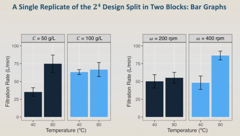
 In the left, we have the temperature-concentration plot, and in the right, temperature-stirring rate one.
Let’s first analyze the effect of the temperature. At the concentration of 50 g/L, the temperature has a strong effect on the filtration rate. By increasing the temperature from 40 to 80 degrees, we can see a high increase in the filtration rate. However, at the concentration of 100 g/L, The temperature has no effect on the filtration rate. The filtration rate is almost the same at 40 and 80 degrees.
In the temperature stirring rate plot, we can see that at 200 rpm the temperature has no effect on the filtration rate. However, at 400 rpm, the temperature has a strong positive effect on the filtration rate. As the filtration rate increases with the increase of the temperature.
Now, the effect of the reactant concentration: at 40 degrees, the concentration of reactants shows a positive effect on the filtration rate. As the filtration rate increases, with the increase of the concentration of reactant from 50 to 100 g/L. However, at 80 degrees, the reactant concentration has a slight negative to almost no effect on the filtration rate.
And finally, the effect of the stirring rate: at 40 degrees there is no effect of the stirring rate on the filtration rate. However, at 80 degrees, there is a strong positive effect, as we increase the stirring rate from 200 to 400 rpm there is a large increase in the filtration rate.
As a conclusion, the combination of high temperature and high stirring rate shows the highest results, the highest filtration rate; at high-temperature the concentration has almost no effect on the filtration rate, so we can work with any concentration, and the pressure does not affect the filtration rate.
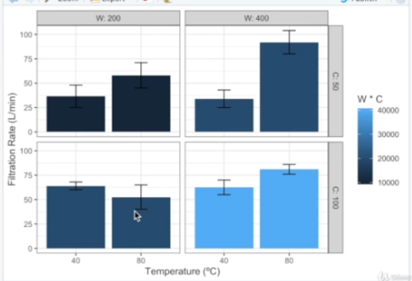 Another way of presenting the experimental data is splitting the results by temperature, stirring rate and concentration at the same time. The main difference between this code and the code from the previous plots is in the facet_grid function. Now we are splitting the plots by concentration and stirring rate. We'll have four plots, one plot for each concentration-stirring rate combination. Let's go to R and run it now. The code here is in the plot temperature, concentration and stirring rate. And let's run it. Now we have four plots, for each concentration and stirring rate combination, 50 g/L and 400 rpm, 50 g/L and 200 rpm, 100 g/L and 400 rpm, and finally 100 g/L and 200 rpm. 50 g/L and 200 rpm, 100 g/L and 400 rpm, and finally 100 g/L and 200 rpm. The resulting graph shows the filtration rate results for each combination of temperature, concentration and stirring rate. The analysis is very similar to the previous graphs, and the conclusions will be the same. Both plot shows the same results, but in a slightly different way. The previous plot shows the factor effects very clearly, while this plot shows the individual results. The choice between one or another depends on the focus one is trying to give to the discussion.