Section 9: Highly Fractionated Designs

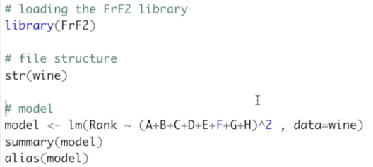
Welcome back, and let’s start our analysis. I have the R code and the data files already opened. The data file shows the eight factors A, B, C, D, E, F, G, and H, and the response variable, the rank. To analyze this fractional design, we’re going to use some functions of the FrF2 package, so let’s load it. Before starting the analysis is always a good idea to check the file structure. We have 16 observations of nine variables, and all variables are numerical. So we can start the analysis.

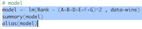
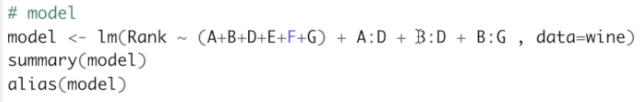
In this analysis, I am going to skip the analysis of variance and go directly to the regression model since the significance of coefficients of the linear model, when using coded variables, are the same from the ANOVA table. Let's start by building a linear model for the main factors and two-factor interactions.

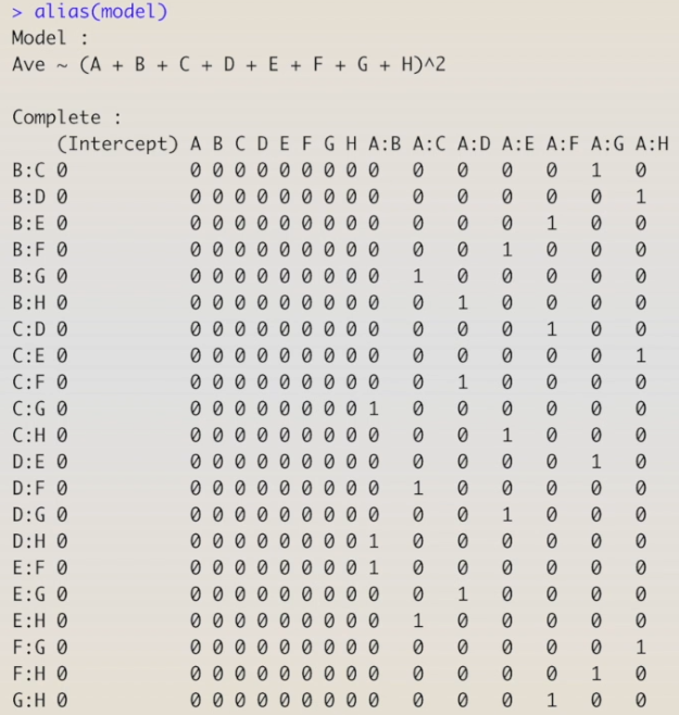
The result shows that most of the interactions were not estimated. This is a fractional design that was divided in half four times, we probably have several interactions aliased to each other. So, let’s take a look at the aliases in this design.

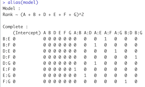
The table shows the aliases among main effects and two-factor interactions, and two-factor interactions among them. We can see the aliases by crossing columns and rows. The number one in the crossing means the factors or interactions are aliased to each other.

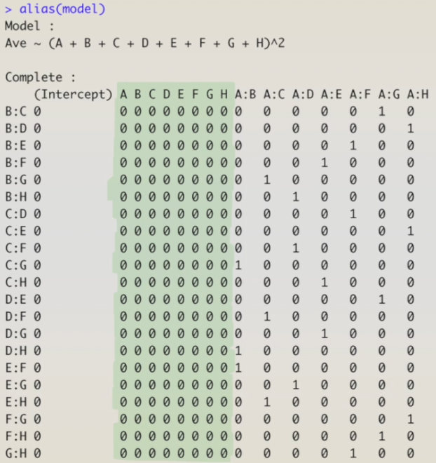
We can see that the main effects are not aliased to any two-factor interactions;

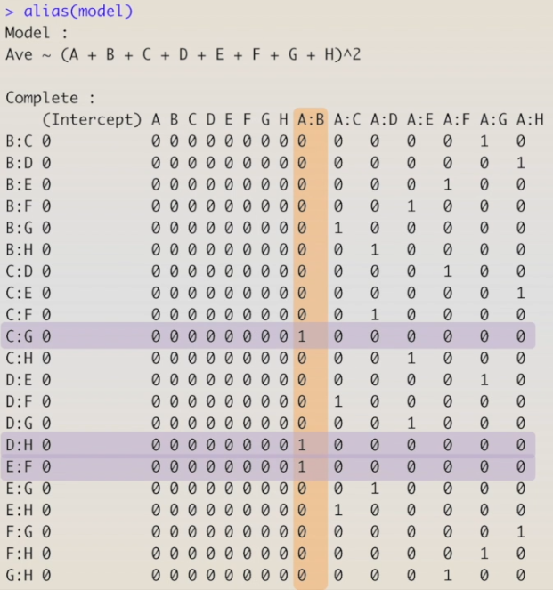
however, each two-factor interaction is aliased to three other two-factor interactions. For instance, AB is aliased to CG, DH, and EF; AC is aliased to BG, DF, and EH; and so on.

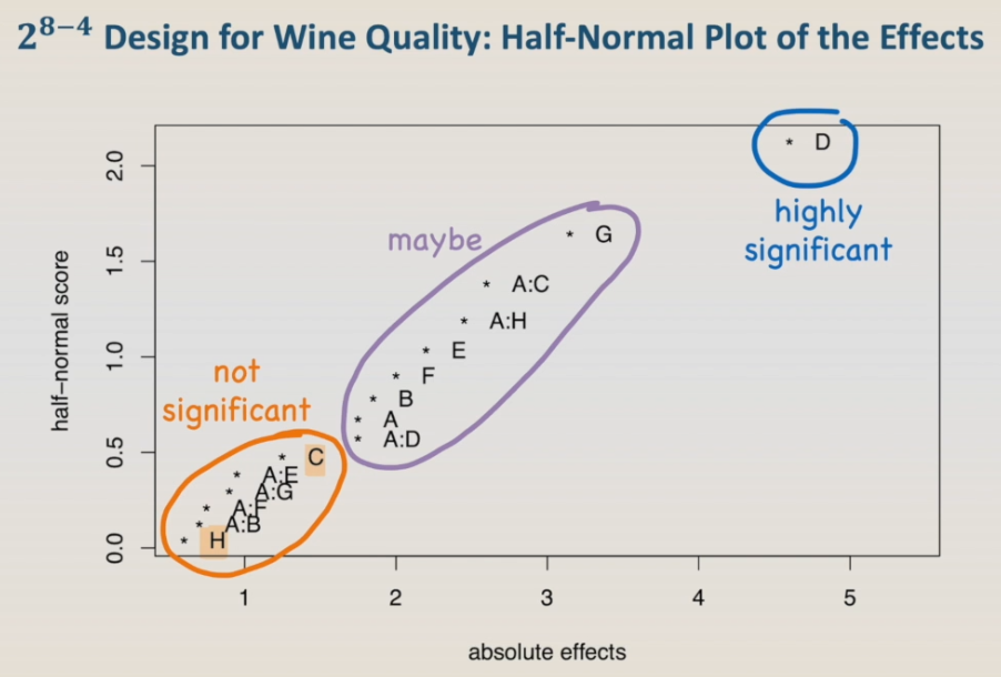
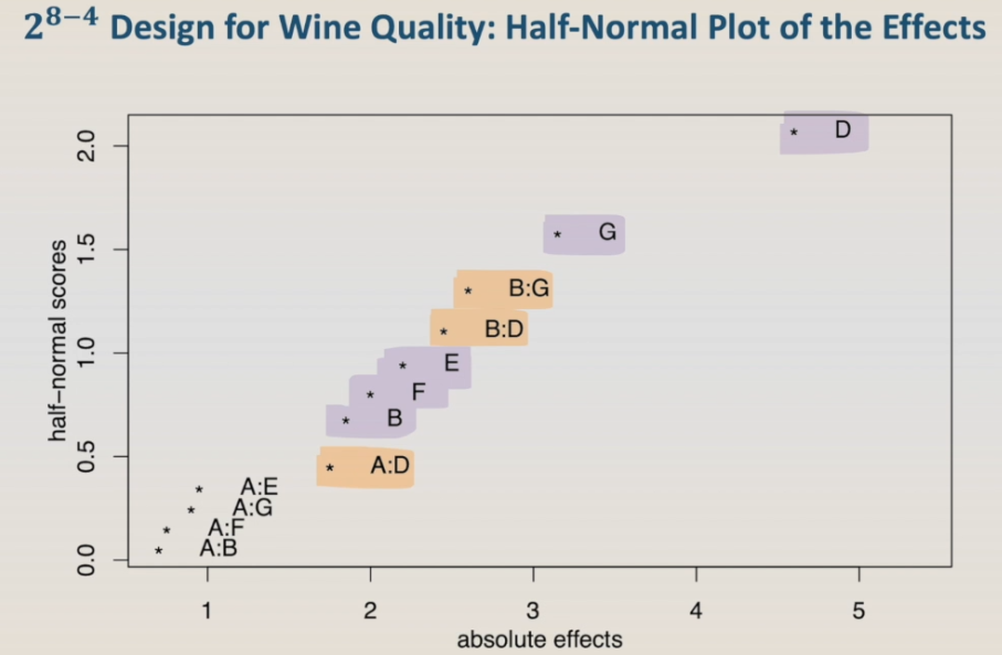
As this is a quite large design, a graphical visualization of the effects can be very helpful in choosing which factors and interactions are significant. One of the best ways of visualizing significant effects is using the half-normal plot of the effects, that is also called Daniel plot. So, let's run it.

The half-normal plot shows all the main effects and interactions that are being tested in the model. In the horizontal axis, we have the absolute effects, and in the vertical axis, the half-normal score. We can visually group the effects and interactions in this plot into three clusters. The ones in the upper right corner, in this example factor D, is the one that is highly significant. The ones close to the origin are the ones that are not significant. And the ones in the middle, that are the ones that maybe are significant. Based on these results, we can see that factor C and factor H are in the group of non-significant effects, so let's remove them from the model and run the model, the alias, and the half-normal plot again.

For this model, the table with the regression coefficients shows some significant effects, and the table with the aliases is way simpler than the previous one. It shows that most two-factor interactions are only aliased to another one two-factor interaction.

Based on the half-normal plot of the effects, in our next model, we are going to keep only the main factors and the interactions AD, BD, and BG. Let's do it.

We need to delete the "power of two" and add the interactions AD, BD, and BG.

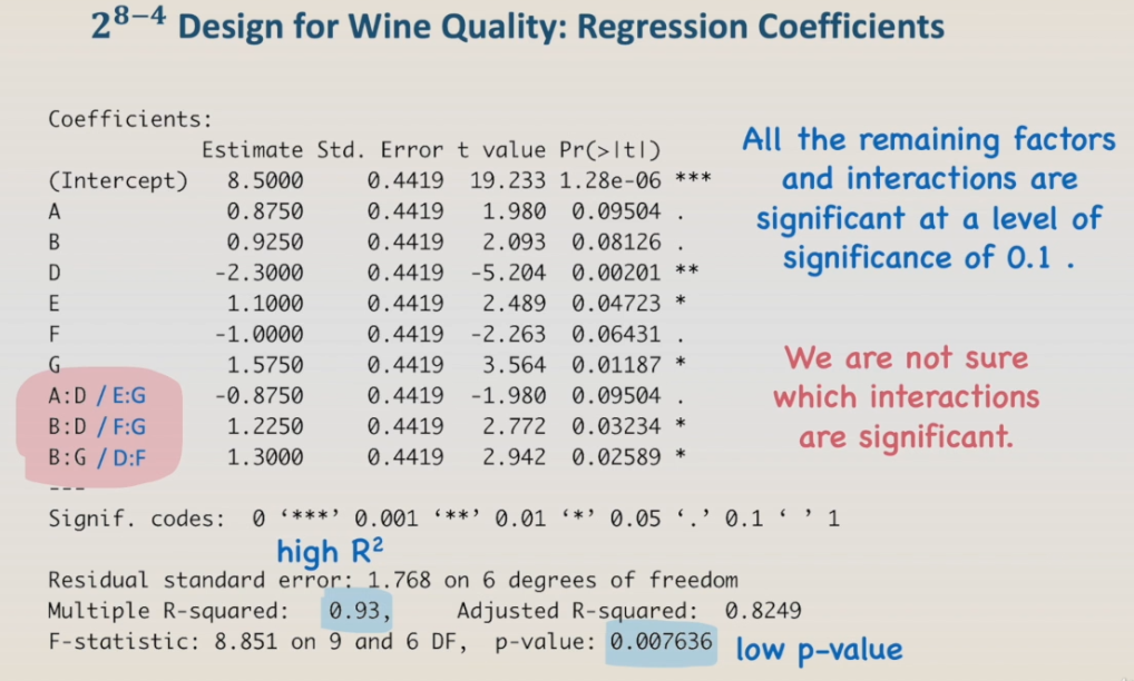
The result shows that all the remaining factors and interactions are significant at a level of significance of 0.1. Also, the model has a high R-squared, 0.93, and a low p-value. If we continue to remove the main effects and interactions from the model, the error term will increase, and the regression terms will not be significant anymore. You can try it by yourself. We have to keep in mind that fractional designs are to be used as screening experiments. Usually, we would not have enough information for final conclusions, but for the choice of factors and factor levels to design the next experiment. For instance, in fact, we don't have enough information to conclude which interactions are significant since AD is aliased to EG, BD to FG, and BG to DF.

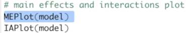
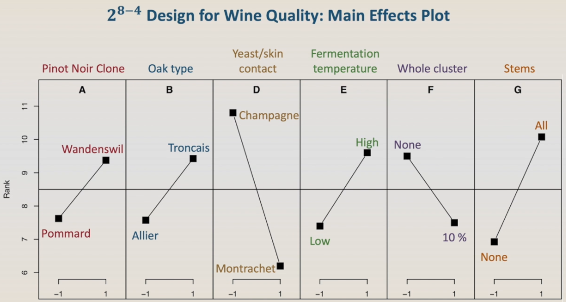
However, the FrF2 package has some other useful tools to help with the analysis, as the main-effect-plot and the interaction-plot. First, let's run the main effect plot. To help with the interpretation, we need to label the plots using the table with the factor's levels. And here we have. Remembering that lower rank is better, the plots show that the best Pinot Noir will be made with the Pommard clone, using Allier Oak type, with the yeast Montrachet, fermented at low temperature, with 10% of whole clusters, and no stems. However, we have to keep in mind that this is a preliminary test and that we have interactions.

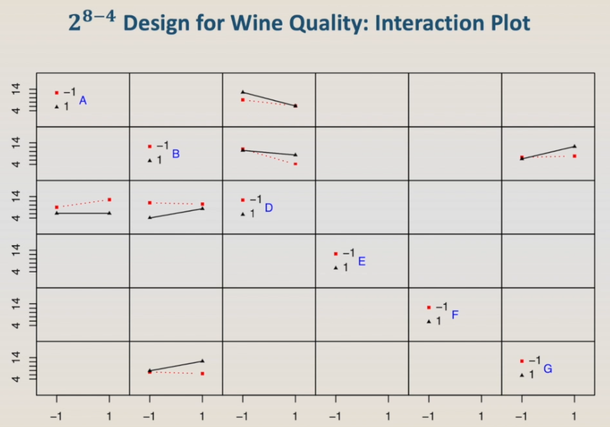
So let's take a look at the interaction plot. The interaction plot interpretation is challenging because we don't really know which interactions we are looking at since there is still aliasing between the two-factor interactions.

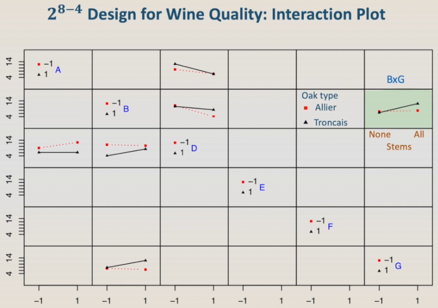
For instance, the highlighted plot can be interaction B:G, stems and oak-type. In this case, for the oak Allier, the presence of stems does not affect the wine rank.

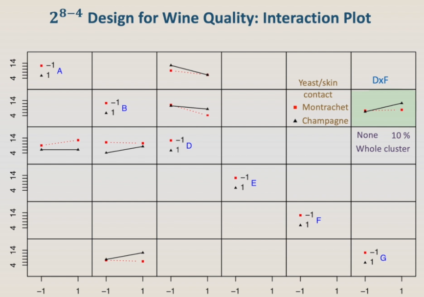
However, it can also be the interaction D:F, yeast, and whole cluster. In this case, for the yeast Montrachet, the presence of the whole cluster does not affect the wine rank. The bottom line is we don't know. We need more experiments to have the answer.

The last step is to build a final presentation of the results, some plot where it is easier to visualise the behaviour of the rank with the studied factors.