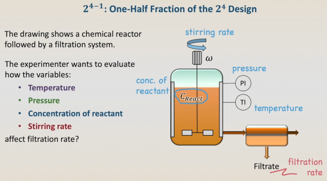
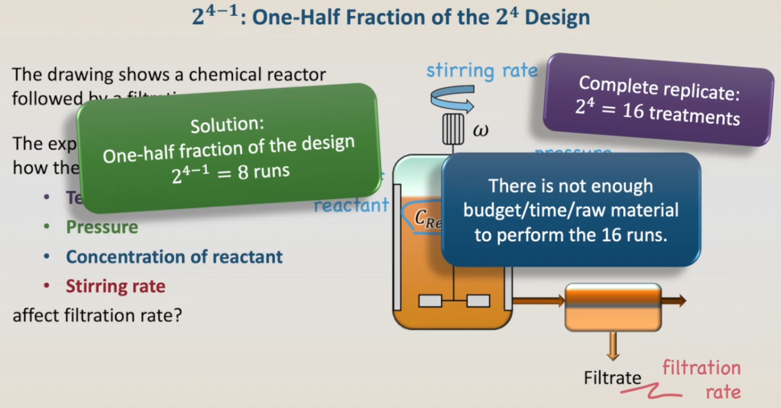
To illustrate the design and analysis of half-fraction designs, let's take again the example of the chemical reactor followed by a filtration system. We want to evaluate the effects of the temperature, pressure, concentration of reactant, and stirring rate on the filtration rate. A complete design involves 2⁴, 16 treatments. However, let's imagine that there is not enough budget, time, or raw material to perform the sixteen runs. The solution is to run a half-fraction of the design, eight runs.

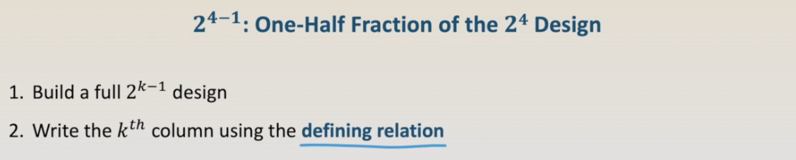
To build the half-fraction design, we have to build a full two in the power of k minus one design and then write the last column by using the defining relation that we don't have yet.

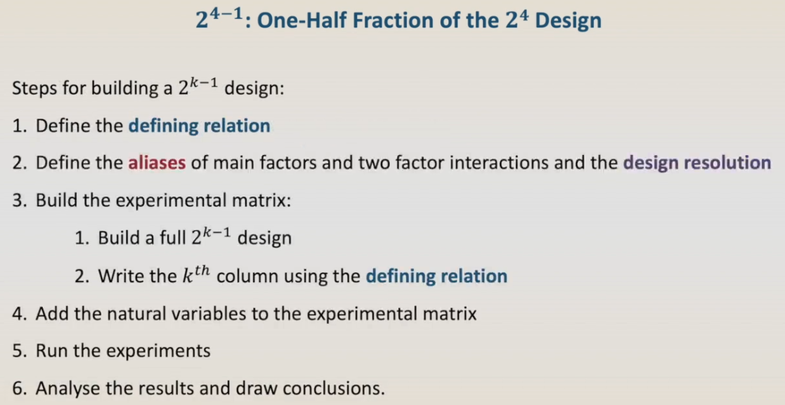
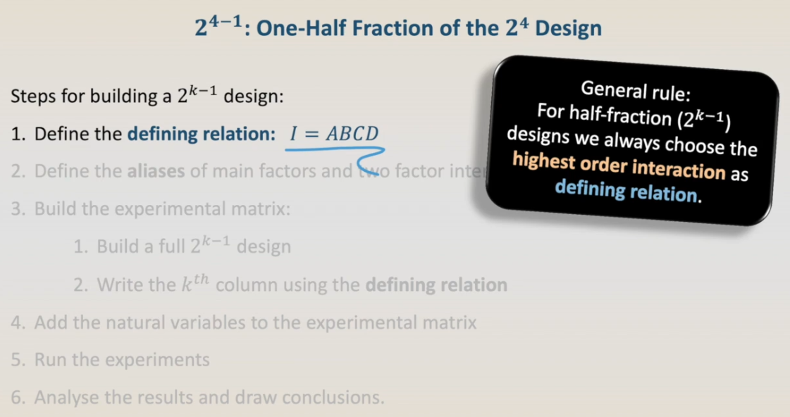
So, let's take one step back and look into the whole procedure of designing and analysing half-designs. The first step is to define the defining relation. With the defining relation, we are going then to define the aliases of main factors and two-factor interactions and the design resolution. Then we're going to build the experimental matrix, to add the natural variables to the experimental matrix, run experiments, and finally analyze the results and draw conclusions.

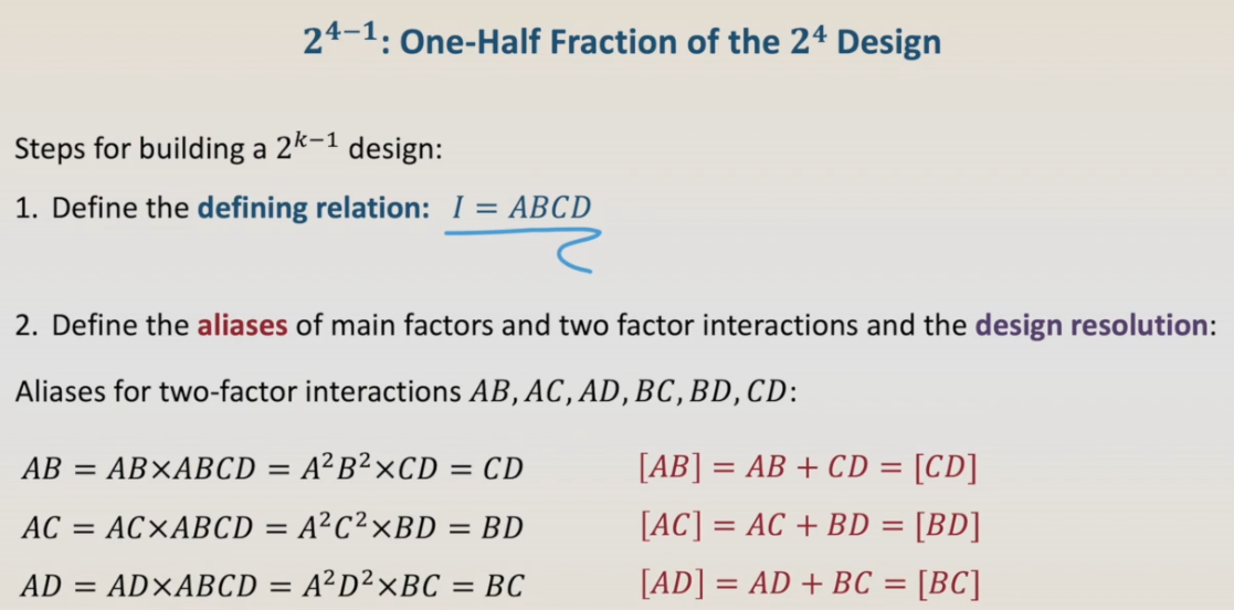
Let's start with the defining relation. As a general rule for half-fraction designs, we always choose the highest-order interaction as defining relation. In this case, identity equal to the four-factor interaction ABCD.

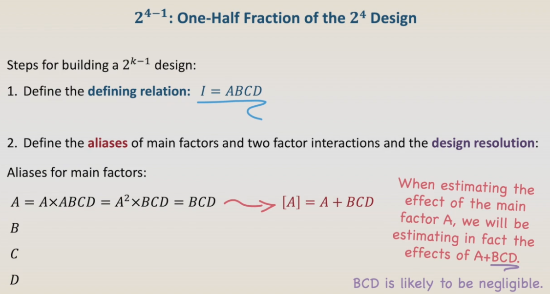
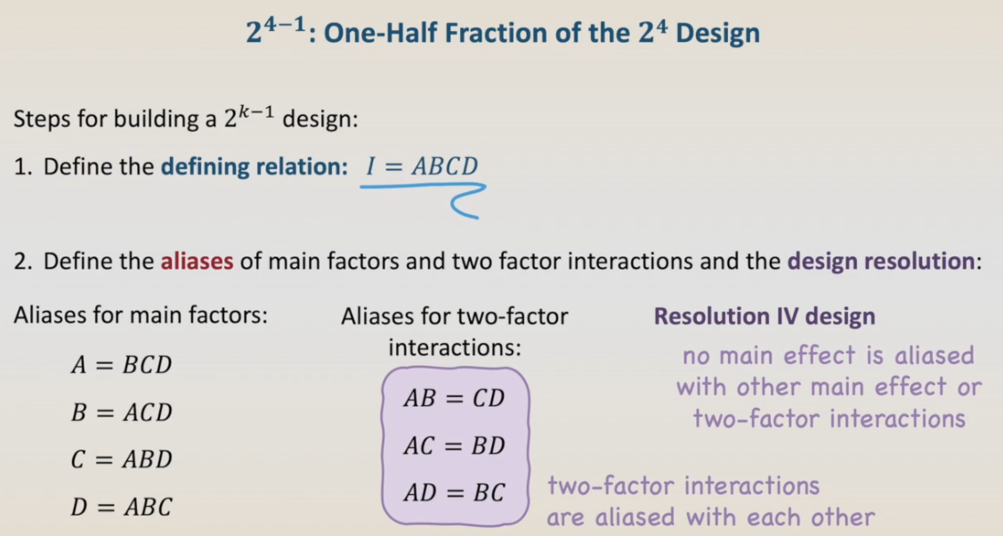
Now we can use the defining relation to define the aliases of main factors and two-factor interactions and the design resolution. Aliases of the main factors A, B, C and D: The aliases of A: A is A times the identity ABCD. This is A to the square times BCD, that is BCD. When estimating the effect of the main factor A, we will be estimating in fact the effects of the main factor A plus the three-factor interaction BCD. However, as BCD is likely to be negligible, we are safe in estimating the effect of A.

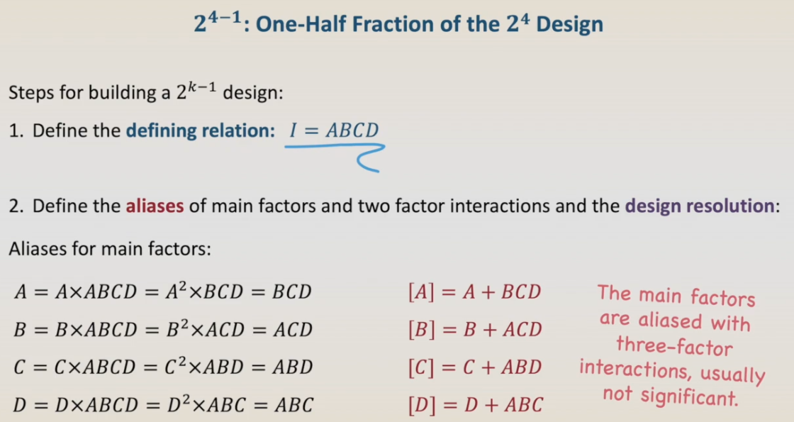
Now, you can pause the video and try to define the aliases of the other main factors by yourself. OK. Let's continue. In the same way as the aliases of A, B is aliased to ACD, C is aliased to the three-factor interaction ABD and D is aliased to ABC. In this design, the main factors are aliased with three-factor interactions, usually not significant.

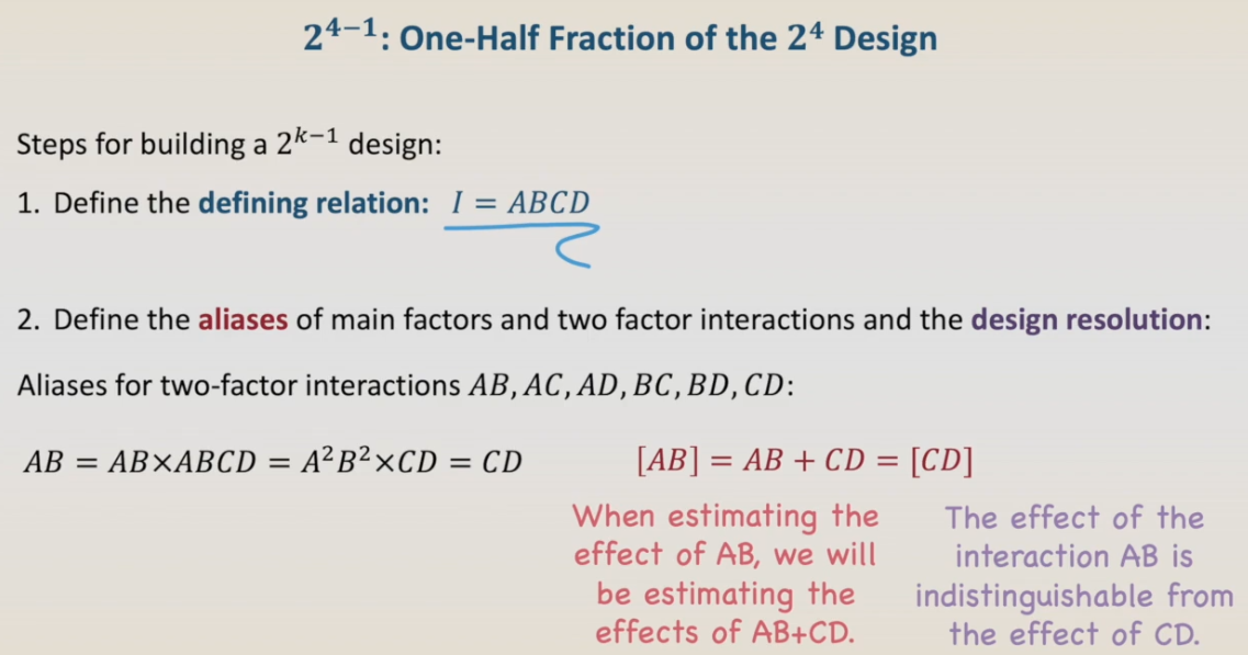
By following the same procedure, we can define the aliases for the two-factor interactions AB, AC, AD, BC, BD and CD. AB is AB times the identity ABCD, that is A to the square, B to the square, CD, that is CD. When estimating the effect of AB we will be estimating the effects of the interaction AB plus the interaction CD. The effect of the interaction AB is indistinguishable from the effect of the interaction CD.

In the same way, AC is aliased to BD, and AD is aliased to BC.

The summary of aliases in this design shows that this is a resolution four design, where no main effect is aliased with other main effect or two-factor interactions; and the two-factor interactions are aliased to with each other.

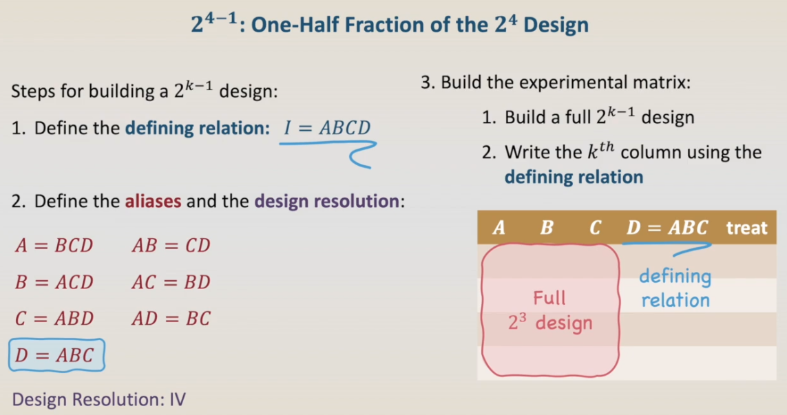
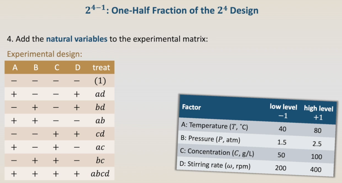
Now we are finally ready to build the experimental matrix. As we have four factors of interest A, B, C, and D, we will start by building a full two in the power of three design and then write the D column by using the defining relation, identity ABCD, in this case, D equal to ABC.

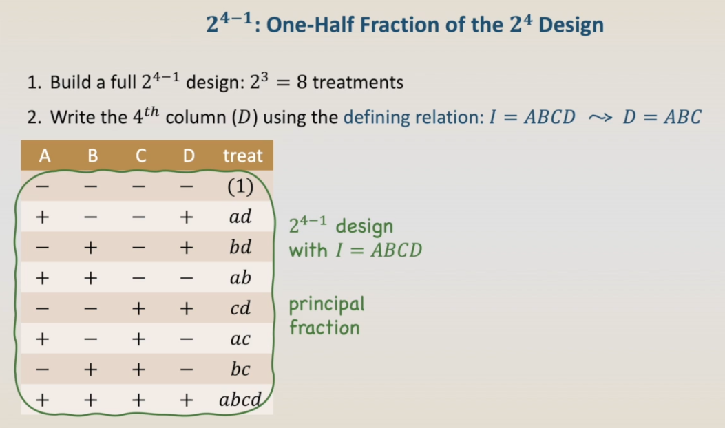
So, let's do it. To build a full two in the power of three design, we'll start by writing at two in the power of two design in the standard order: for factor A, minus plus minus plus, and for factor B, minus minus plus plus. Then we duplicate it and assign minus signs to the upper half of column C, and plus signs to the lower half of column C. This way we have a full two in the power of three design. Now column D will be given by the multiplication of column A times column B times column C.
For the first row: minus times minus is a plus, times minus is a minus; we have a minus, that is treatment one. For the second row: plus with minus is a minus, times minus is a plus, we have treatment ad.
For the third row: minus with plus and minus is a plus, treatment bd;
plus with plus and minus, we have a minus, ab;
minus and minus with a plus is a plus, treatment cd;
plus and minus plus is a minus, ac;
minus plus and plus is a minus, bc; and
finally plus plus and plus will be a plus, this is treatment abcd.
Now we have the principal fraction of a two in the power of four minus one design with identity ABCD.

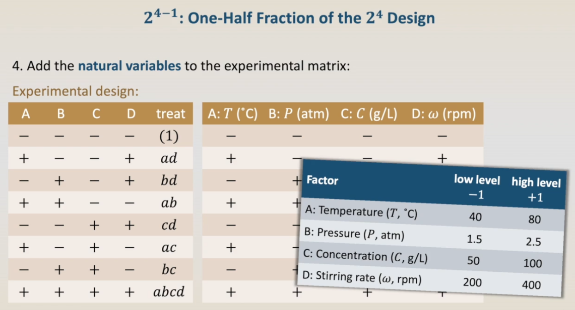
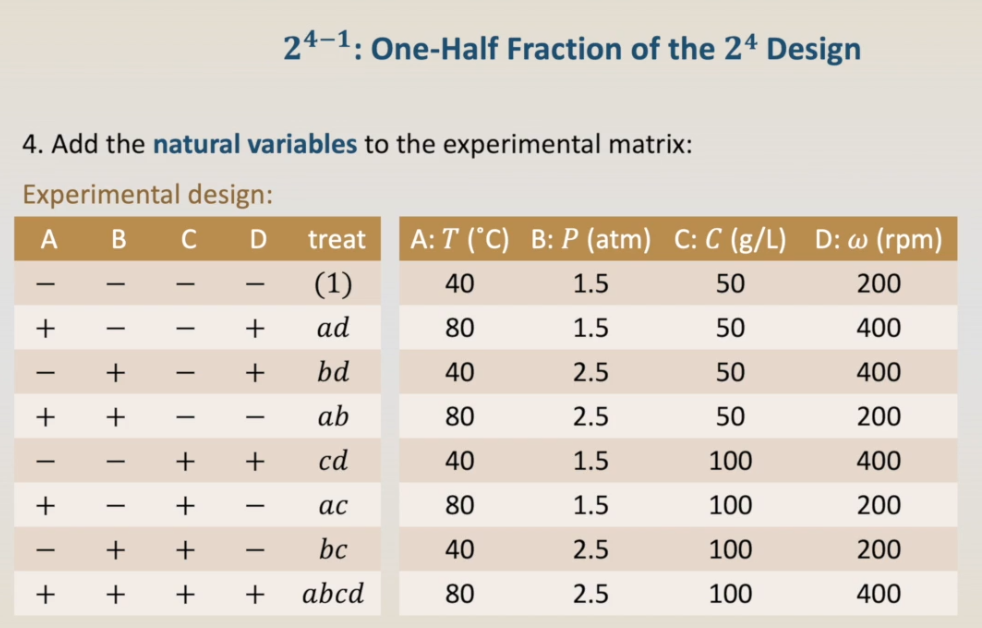
The next step is to add the natural variables to the experimental matrix. In this design factor A is temperature, the low level is 40 and the high level is 80 degrees. Factor B is pressure, one point five and two point five atmospheres. Factor C is the concentration, fifty and hundred grams per liter, and factor D, the stirring rate, two hundred and four hundred rpm. Here we have the table with temperature, pressure, concentration and stirring rate. For the temperature, the minus sign or low level is 40 degrees and the plus sign is the high level or 80 degrees; and the same for pressure, concentration, and stirring rate.

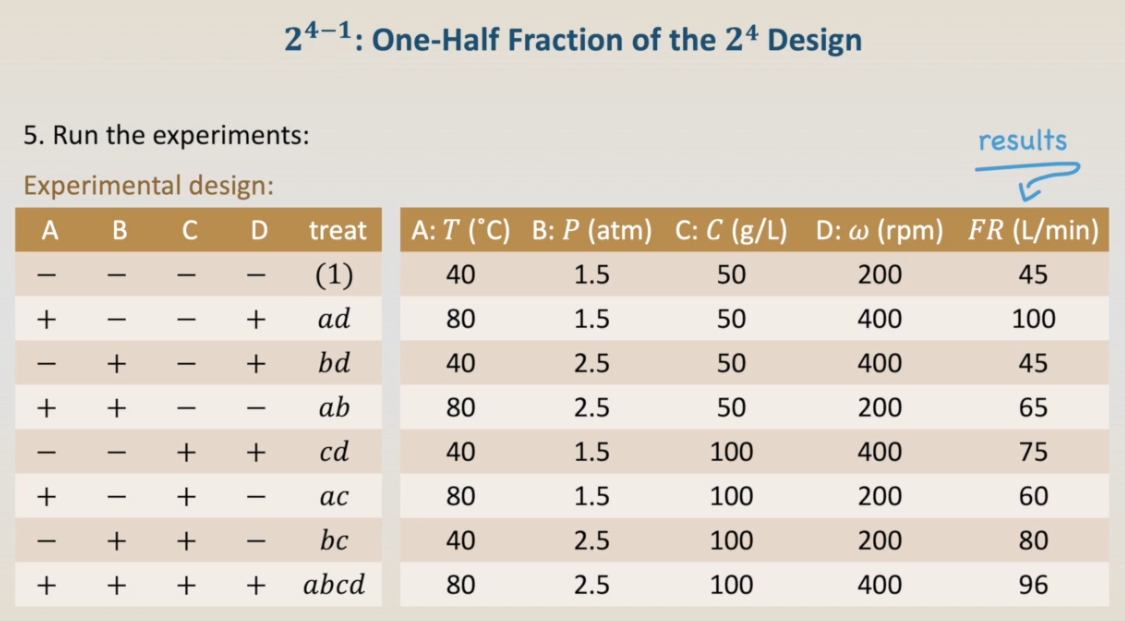
Now we have to randomize, run experiments, here we have the results, and then analyze and draw conclusions.