Section 7: Blocking a Factorial Design
Let’s start our analysis by opening the csv file. Let’s start our analysis by opening the csv file. In this data file, we have the columns for the coded variables xT, xP, xC and xW. We have also the natural variables temperature, pressure, concentration and stirring rate. We have a column for the blocks and then we have two columns for responses, filtration rate one and filtration rate two. The results in this example are the filtration rate one, FR1, that is the one that we are going to use in our analysis.
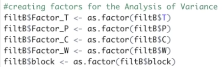
Now, let’s check the file structure: We can see here that we have 16 observations of 11 variables and all variables are numerical. To run the analysis of variance, we need variables as factors. So let’s create factor T for temperature, factor P for pressure factor C for the concentration, factor ω for the stirring rate; and for the block we are not going to create a new variable, but we are going to transform the existing one, block, as as numerical to factor.
 We can do this because we are not going to use the blocks in the regression model, then we don’t need to keep the blocks as numerical.
So let’s run the code. Now we have four more variables, Factor_T, Factor_P, Factor_C and Factor_omega. And these new variables are defined as factors with two levels each, as are the blocks. The block now is a factor variable with two levels.
 Now, let’s run an analysis of variance with the response filtration rate one, by taking to account the blocks and all the main factors and two-factor interaction, three-factor interaction and four-factor interaction between factor T, factor P, factor C and factor ω.
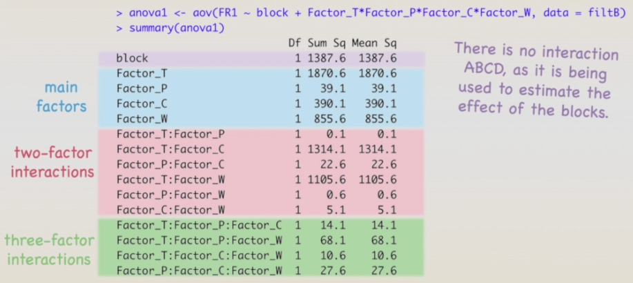 Let's run it. Here we have `the resulting analysis of variance` table. We can see the blocks, the main factors, the two-factor interactions and the three-factor interactions. We can see the blocks, the main factors, the two-factor interactions and the three-factor interactions. There is no four-factor interaction ABCD, once it is being used to estimate the effect of the blocks. We don't have the F-zero and the p-values yet. Since this is a single replicate experiment and it doesn't have the degrees of freedom to estimate the residuals.
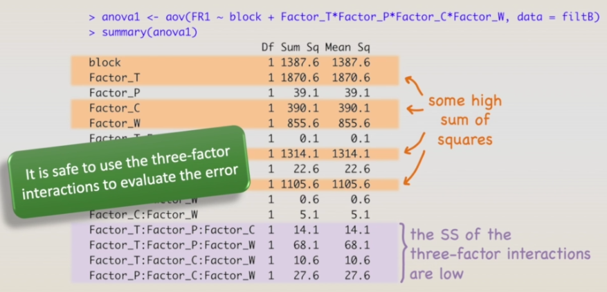 However, we can take a look in the sum of squares. We have some high sum of squares and compared to them the sum of squares of the three-factor interactions are low. So it is safe to use the three-factor interactions to evaluate the error.
 Now let's run a new `analysis of variance` by taking into account the blocks, the main factors and the two-factor interactions, and the three-factor interactions will be used to estimate the error. Let's run our second analysis of variance.
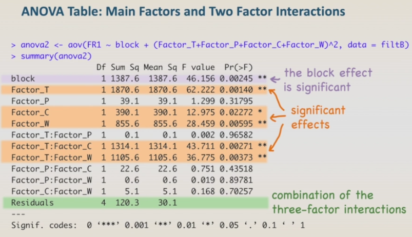 The resulting analysis of variance shows that the block has a significant effect on the results, as have the temperature, the concentration, the stirring rate and the interactions between temperature and concentration, and temperature and stirring rate. The residuals are formed by the combination of the three-factor interactions.
By performing backwards elimination of the non significant effects we can have a final ANOVA table with only the significant effects. You can stop the video now and try doing it by yourself. It is the same procedure we have already done previously.
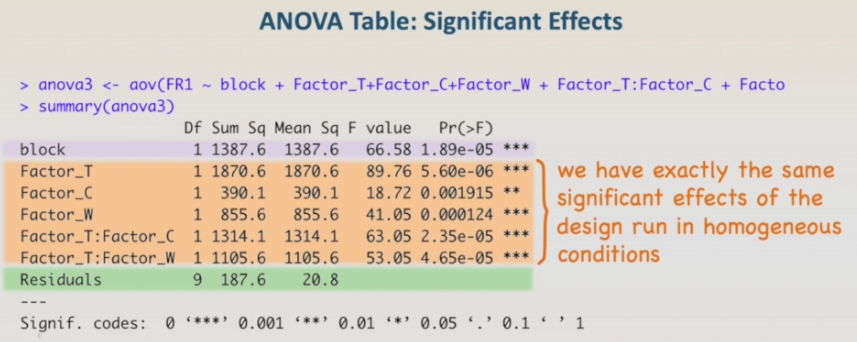 I will skip directly to the final ANOVA table with only the significant effects. The final ANOVA table shows exactly the same significant effects of the design run in homogeneous conditions, plus the effect of the blocks and all the effects are highly significant with very low p-values. conditions, plus the effect of the blocks and all the effects are highly significant with very low p-values. As next step we are going to run the regression models and check for the model adequacy.