Section 3: Factorial Designs

Let’s take a look in this example of a two-factor factorial experiment with both factors, A and B, being tested at two levels each. We call these levels low and high, and we use the minus and plus signs to identify them. To make it easier, let’s take the example of the effect of the route and the hour of the day on the total time to commute from home to work. In this case, Factor A is the time we leave home, can be seven or eight a.m.. Factor B is the route we take, R1 or R2, and our response is the commute time in minutes.

The effect of a factor is defined as the change in the response produced by a change in the level of the factor. We call it main effect because it refers to the primary factors of interest in the experiment. In our example, the effect of factor A, the time we leave home, is the average commute time we take when we leave at eight a.m., minus the average time when we leave at seven a.m., 21 minutes. In the same way, the effect of the route is the average time we take when we use route 2, minus the average time when we use route 1: 11 minutes. The effects graph can easily illustrate this behavior. Here we see that leaving that eight a.m. causes an average increase of 21 minutes in the commute time compared to seven a.m. and using route two causes an average increase of eleven minutes in the commute time compared to route one.

In some experiments we may find that the difference in the response between the levels of one factor is not the same at all levels of the other factors. In this modified example, the leaving time has a positive effect when using route 1, meaning that we take more time to go to work, if we leave at eight a.m., but the leaving time has a negative effect when using route 2, meaning that we take less time to go to work if we leave at eight a.m.. Because the effect of the leaving time depends on the route we say that there is an interaction between them: the effect of the leaving time at route 1 is 30 minutes, and the effect of the leaving time at route 2 is -28 minutes. 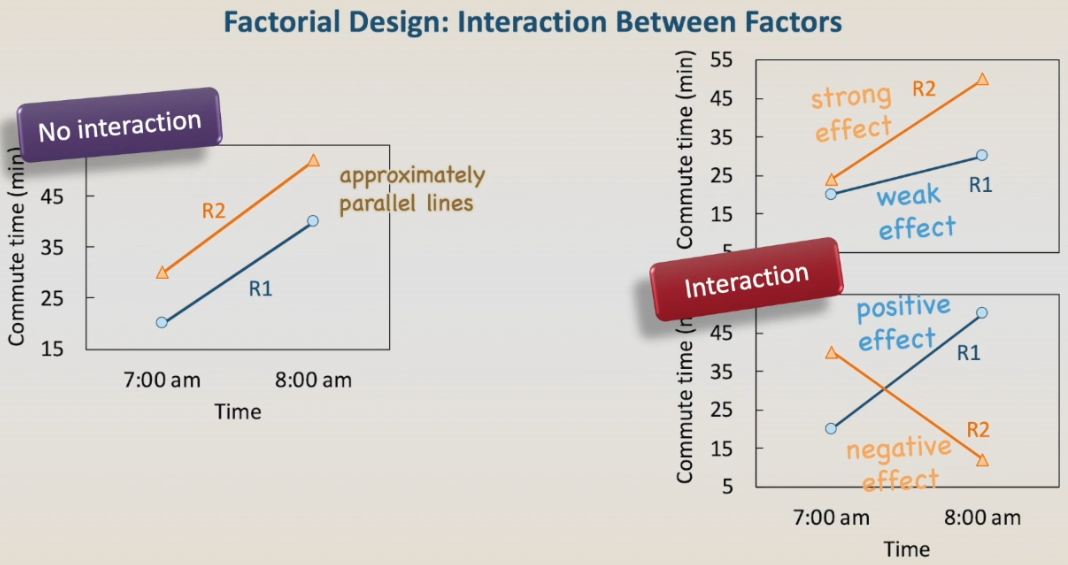Interactions between factors can be easily spotted in graphs, in the graph on the left, the increase in the commute time by leaving that eight a.m. is roughly the same using either route one or route two, there is no interaction and the lines showing the effect of the leaving time are approximately parallel. However, the graphs on the right tell a completely different story. In the upper graph, the living time has a weak or small effect when using route one, but a strong effect when using route two. In the lower graph, the leaving time has a positive effect when using route one, meaning the commute time increases by leaving at eight a.m., and has a negative effect when using route two, meaning the commute time decreases when leaving that eight a.m.. In both cases, the effect of the leaving time on the commute depends on the route, showing a clear interaction between them.