Section 2: Experiments with a single factor
For the analysis of variance it is useful to describe the observations using a statistical model.
\begin{equation}
y_{ij} = \mu + \tau_i + \epsilon_{ij}
\end{equation}
Hypotheses test: \begin{equation} H_0: \tau_1 = \tau_2 = … = \tau_a = 0 \end{equation}
\begin{equation} H_1: \tau_i \neq 0 \end{equation}
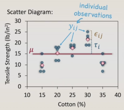
In the effects model Each observation yij can be represented by an overall mean, μ, plus the effect of the ith treatment, $\tau_i$, plus a random error, $\epsilon_{ij}$. The effects model is not the only model to be used to represent the data. However, it has some intuitive appeal in that the average μ is a constant, and the treatment effects $\tau_i$ represent the deviation from this constant when the specific treatments are applied. This model is called `single factor analysis of varianc`e or `one-way ANOVA`. As the treatment effects can be considered as a deviation from the overall mean, The hypothesis test for the one way analysis of variance can be expressed in terms of the treatment effect $\tau_i$. In the null hypothesis $\tau_i$ is equal zero for every i. That is the effect of the factor is zero, there is no deviation from the overall mean. In the alternative hypothesis H1 $\tau_i$ is different from zero for at least one i, meaning the cotton content affects the tensile strength, at least at one level of cotton content.