Section 2: Experiments with a single factor

In the previous section, we have discussed methods for comparing two conditions or treatments. The example analyzed two cement formulations, with or without polymer. Another way to describe this experiment is as a single factor experiment with two levels of the factor. However, many single factor experiments involve more than two levels of the factor. This section focuses on methods for the design and the analysis of single factor experiments with an arbitrary number of the levels of the factor.

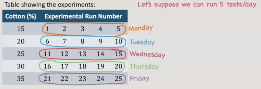
We are going to start directly by analyzing an example that is the development of a new synthetic fiber that will be used to make cloth for men’s shirts. The objective is to maximize the cloth tensile strength. The tensile strength of a fabric is the measure of the maximum pulling force it can support before it breaks. From previous experience, we know that the tensile strength is affected by the weight percentage of cotton. We also know that probably any increase in the cotton content will increase the tensile strength and that the cotton content should range between 10 and 40% due to limitations in the process. This way, it was designed an experiment to test 5 levels of cotton content, between 15 and 35% with five replicates. This is an example of a single factor experiment where the number of levels “a” is five. The number of replicates “n” is five also. And we have a total of 25 observations. Let’s suppose we can run only 5 tests per day. Thus, we can run all the experiments with 15% on Monday, The experiments with 20% on Tuesday, the ones with 25% on Wednesday. On Thursday, the ones with 30%. And finally on Friday, the ones with 35%. However, this is a really bad way of organizing and running the experiments, since the effect of the cotton percentage is confounded with the day. But why this is a problem? We don’t know. Maybe on Tuesday there was a problem with the scales and all the samples that should have 20% had 22. Maybe the relative humidity on Wednesday was higher. And the fact that the measurements of the tensile strength, or maybe even the experimenter had some personal issues and was distracted on Monday. The bottom line is we don’t know. That’s why we have to randomize the tests, meaning that the experiments should be run in random order, guaranteeing that the experimental noise is equally distributed among the runs. 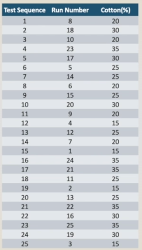An efficient way to generate the random order is to enter the 25 runs in a spreadsheet like Excel and generate the column of random numbers using the RAND() function. Or we can always write the test numbers in small pieces of paper, fold and sort. The table on the right shows the randomized test order. This random test sequence is needed to prevent the effects of unknown noise variables, perhaps varying out of control during the experiment, from contaminating the results. The table on the left now shows the experimental results.

It is always a good idea to examine experimental data graphically. The figure on the right shows the scatter diagram where we can easily see the noise or variability of the results. We can also see that between 15 and 30% there is an increase in the tensile strength with the cotton content. And after that, a sharp decrease. However, we wish to be more objective in our analysis of the data. Specifically, suppose that we wish to test for differences between the average result of each level of cotton percentage. The appropriate procedure for testing the equality of several means is the analysis of variance. is the analysis of variance. However, the analysis of variance has a much wider application than the problem above. It is probably the most useful technique in the field of statistical inference.