Step 1: Compound optimization
- Q1 scan (identify the parent)
- Product ion scan (identify the fragments)
- MRM scans (optimize your parameters)
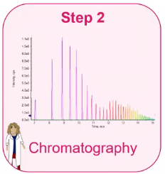
Step 2: Chromatography
- Choosing a column
- Selecting a mobile phase
- Using chromatography
Step 3: sMRM method
- Run a mid or high level standard
- Create a method in analytics and process a sample
- Copy and paste RT into your method
Hello, and welcome to the second session of LC-MS/MS 101 method development. Today we’re going to focus on strategies and techniques for method development for mass spectrometry assays. I’m Crystal halt, and I’m your moderator for today. Today I’m joined with our speaker Dr. Karl Oetjen. Dr. Karl Oetjen, is a senior scientist driving food, environmental forensics, clinical and cannabis applications at science. Before joining science, he completed his PhD at Colorado School of Mines, where his research focused on non targeted characterization of complex surfactant mixtures, including aqueous film forming foams, which led to the discovery of several novel per and polyfluorinated alkyl substances, also known as PFS, that since it’s been found in a variety of environmental samples, and industrial chemicals. Since joining sciex, Karl has worked with numerous labs, creating and implementing both quantitative and qualitative methodologies. Take it away, Karl.
Thank you so much, crystal. So if you’re new, or just joining us today, welcome. If you’re returning, that’s awesome. Glad to have you here. And we’re gonna be talking about method development. So method development is really the time that we get to be a little bit creative as analytical chemists. So we’re going to cover the approach to making a new quantitation method. So this would be for a new assay, just from scratch. But also the same steps could be used to add a compound to an existing assay, just something we get asked a lot to do.
Step 1: Compound optimization #
So up first, we’re going to be talking about compound optimization.
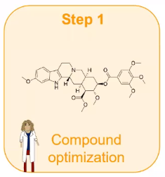 So this is going to be our sort of first thing we need to do, we need to define what our compounds are, we need to choose what compounds we want to look for. And then we need to optimize for those parameters. So the method we’ll be building today will be a quantitative method. So this will be a standard MRM method.
So up first, we’re going to go ahead and identify a product or do that Q1 scan. So if you remember from the previous session, when we were talking about parents, the parent is what we’re interested in. So that say, if we are interested in Reserpine that is what we’re going to be looking for. So we first need to identify it. So we’re going to do a Q1 scan, which is going to scan an area and we’re going to talk a little bit about how to set that up.
Next, we’re going to define the fragments. So we talked a lot last time about fragmentation, fragmentation methods. So those fragments are sort of like the compounds fingerprints. And in MRM experiment, if you remember, we’re going from a parent to a daughter or a precursor to a fragment. So we really need to first define what fragments exist for that compound.
And last, and probably most important, we need to optimize parameters for the specific fragments.
Slide #
[3:17] So let’s get started. So the first thing we need to decide is what ionization technique we’re going to use.
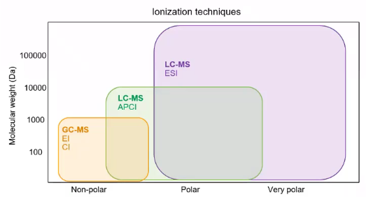 So LCMS, right, we’re mostly talking about electrospray ionization, that’s the probably the most commonly used ionization technique. But within ESI, there’s positive and there’s negative. There’s also APCI. So if you are dealing with compounds that are a little nonpolar, maybe sort of with that GC realm, maybe APCI will be a good choice, we’re going to talk a lot about ESI. And pretty much exclusively, but I like to use this example, as a time when Hey, APCI was actually a better choice. So for this compound, Irganox 1076, I went ahead and ran it four times the same instrument with the same column, the same standard, and I just changed the ionization techniques.
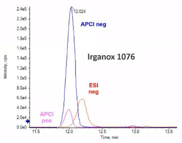 So I went from an ESI negative mode to an API and negative mode. did subsequently in positive mode, as well. And what you see is you get this really nice giant peak for APCI negative. This kind of makes sense for this compound. It’s got a really long alkyl tail. But for ESI, you get a much smaller signal and for use that positive sentiment shown because there really wasn’t a signal. So we’re going to want to take some time to sort of consider the analysts were interested in. So what are their size? How polar are they? Were they traditionally done by GCMS? Before we kind of move into our ionization approaches, but for the majority of the time, if not more than 95% of the time, we’re going to be dealing in the ESI realm.
Slide #
So what’s the difference between positive and negative, and just put very simply, the difference between positive and negative would be in positive mode, we’re really adding something. So here we’ll be adding maybe an ammonium, or a sodium. And we call these things adducts, or a +H would be the common was common adduct that you’d observe. So in positive mode, we’re adding something to our compound. So even if your your compound has been true mass of, let’s say, 100, if we add a +H, the observed mass would be 101. Right? Because we’re adding something that compared to negative mode, where we’re, we’re taking something away. So in negative mode, we would be, for example, removing hydrogen, so we’d see a -1. So if that same compound had a mass of 100, our observed mass would be 99. And that’s really why we have to do this Q1 scan, you need to observe what the mass we want to isolate for MRM experiment. And we have to identify what that mass is.
Slide #
So for this example, I have a polyethylene glycol, and I’m showing you this because we have the +H and the +NH4 adducts shown. So this would be just our simple Q1 skin, I knew the mass of this polyethylene glycol, and I just scanned from a range of 414, up to somewhere around 440.
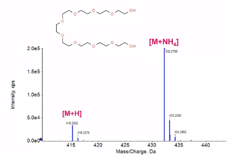 And what I see is kind of interesting. If I were to just go ahead and assume that my +H was the most abundant addict, I’d really miss out on this big NH4 peak. So that p+NH4, which has a lot more sensitivity, or a lot more intensity than this +H. So that’s where sort of doing these definitions of what I’m actually looking for become really important. So with positive mode, which is what we’ll talk about, primarily, we’ll talk about negative mode a little bit, you’ll commonly see +H, +NH4 +Na, so we want to keep our eyes peeled for those +1, +17, +23, of our parent compound versus in negative mode, where most of the time we’re just looking at a deprotonated compound.
Slide #
So just as a little bit of a reminder, from last session, we’re building our MRM method. So the first thing we need to do is identify our parent. In this case, we have a parent of 215. So our quadrupole is going to filter out everything that’s not 215, we then need to go ahead and create some fragmentation. So we’re going to do that in Q2 where the collusion cell. So fragmentation is going to take place. And that will be our next step, we need to define those fragments, what are those masses that that compound fragments into. And then finally, our Q3 will be used as a filter, again, to filter out a specific item in this example would be that 185. So that’s great. That’s a nice little animation of you know, what’s happening, but what are the parameters we’re really after.
Slide: Optimize three major parameters #
And we’re really after these three major parameters,
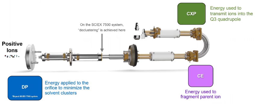
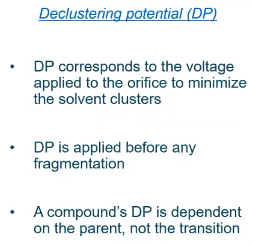
the declustering potential (DP). So if you remember, that’s the ability to, or the energy used to minimize soften clusters. So that’s really going to depend on the parent mass, or the parent compound, rather,
the collision energy (CE). So that’s that energy we’re using to create fragmentation, and then
the collision exit cell potential (CXP). So that would be the energy used to transmit ions through Q3.
So these are the three things that we’re going to optimize for each one of those transitions.
Slide #
But we first have to know what we’re looking for. So I’m going to use the example for Reserpine. Reserpine has a mass of 608. So this massive 608, great, we’re happy. What am I going to do? How do I how do I decide? Or how do I identify what to actually isolate or filter on Q1? So the experiment I’m going to do is called a just a Q1 scan. And essentially what we’re doing is instead of having that quadrupole fixated on a specific mass, we’re letting it scan and mass range. And typically I like to let that mass range be plus or Morocco plus in the case of positive mode 25 Dalton’s from whatever it may be true, massive my compound is and I’m doing that because I want to include all of those adducts, so I want to include that +H that ammonia adduct that put 17 and that sodium adduct that plus 23, says those are the more common adducts that I would observe. So when I do that for Reserpine, I see I get a really nice peek at my plus one. So we’ve protonated this we have 609 now. And that’s what I’m going to choose for my subsequent experiments, because it’s giving me the best density. So I’ve identified my parent.
Slide #
And the next step is to really figure out what is it going to fragment into. So to do that, we’re doing a product scan. So we’re kind of moving our way down the quadruples, as I like to say. So we’ve decided what our Q1 is going to look for. Now we need to get Q2 involved, and we got to create some fragments. So product ion scan, we’re going to filter for just that 609, determined that’s the best. Best to filter out, it’s gonna be the best sensitivity. Now we got to figure out what fragments this was Reserpine make. So we are going to essentially have our Q3 scan from up 50 daltons, since that’s a nice lower limit for a particle up to plus one of our parent mass. So we determined that our observed Mazda 609, so I’m gonna have Q3 stuff at 610, just because I like to see that parent mess in my MSMS spectrum. And it’s just gonna scan that range, and we’re going to read all the fragments. So as we ramp our collision energy, we see fragmentation. So we typically will ramp collision energy, right, because we don’t know what an optimal collision energy is, for any of these fragments. We haven’t done that experiment. So instead, we’re going to ramp it. And we’re just going to observe what happens. And what I like to do is pick the top five fragments, it’s a little bit of overkill, someone say, but usually, if you choose five, you’re in a pretty good place in case one of them has a matrix interference, as you kind of move down in your method development stage. So it gives you a little bit of wiggle room, if you don’t have five fragments, which happens all the time. For example, in the case of fluorochemicals, typically, we only have one maybe two fragments take which can get. And then over five is usually a little bit of a little bit of overkill. But everything we do from this point on is it going to take any more time, if we do it with five fragments, or if we do it with two fragments. So having an extra just gives you a little bit of flexibility in the long run.
Slide: Optimize the declustering potential (DP) #
So we’ve picked our fragments, so we’re going to do our MRM experiment.
 And we’re going to optimize for those parameters we talked about earlier. So the first one would be
 the declustering potential. So the declustering potential right, is the voltage to minimize the solvent clusters. So it’s before any fragmentation is occurring. It’s right at our source, it’s what’s kind of I like to say pulling our compound in.
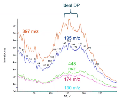 So because of that all of our MRM transitions shown here should look the same. In the sense, the profile should look the same. So we have those five fragmented shows that 397, the 195. And we have their profiles, and we sort of see this decrease by by a little bit of an increase in this sort of level areaish, before it decreases again. And that’s great, too, is dependent on the parent, all of these should look exactly the same. So if I was going to choose an optimal DP value, choose something in this range, probably around 150ish would be a great value for Reserpine. But why did I bother doing this with all of those fragments, if it’s going to be the same? And as based on the parent? What’s the point?
Slide #
And the reason I like to do this kind of a personal preference, but I like to use it as a little bit of a forensic tool.
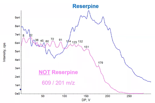 So because we’re looking at fragments of a parent, and that parent should react the same way to declustering potential every time, if we see a different profile like the one shown here in pink, I can go ahead and say, Hey, turns out, maybe maybe I chose a fragment that was really in the mud was very low in intensity, or maybe I have some background ion that’s also has an 609 is giving me sort of this interference, or false peak. And I choose that as one of my fragments I can use to declustering potential as sort of a sanity check to make sure, hey, that profile and pink is very different than the one I saw in blue. And because of that, I can go ahead and say no, that’s not Reserpine. So I’m not even going to consider it, I’m going to remove it. Or maybe this would be a good time for me to go back and, and refuses to serve you and say, Hey, I’m confident this is Reserpine right. So it can be a little bit of a, a tool that you can use to make it so you don’t make any mistakes in the long run. Save yourself a little bit of time. So we’ve written down our declustering potential, that’s going to be the same for all of our fragments,
Slide: Optimize the collision energy #
we chose 150 Now we’re going to go ahead and ramp that collision energy.
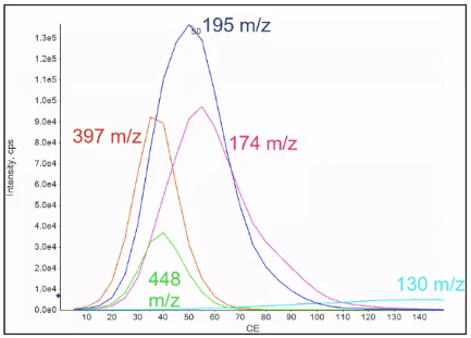 So when we ramp the collision energy, we’re going to ramp it for each one of the MRM transitions are each one of those fragments. Each of them are an experiment individually, and typically will ramp it somewhere from five volts up to 150 And when we do that, what you usually see is that things with smaller fragments require a little bit higher collusion energy, it’s not always true, but it’s a good rule of thumb. So as you increase the collision energy, you’ll start to see smaller and smaller fragments.
So I’ve done that here, each one of these represents my five fragments I chose in the earlier slide, I can go ahead and choose my ideal collision energy. So for that 195 would be about 50, compared to that 174, which may be the 60 range. And I’d go ahead and transfer all these values to a notebook or Excel or however right into my method, however, you’re sort of keeping your notes.
So when we ramp the collision energy, we’re going to ramp it for each one of the MRM transitions are each one of those fragments. Each of them are an experiment individually, and typically will ramp it somewhere from five volts up to 150 And when we do that, what you usually see is that things with smaller fragments require a little bit higher collusion energy, it’s not always true, but it’s a good rule of thumb. So as you increase the collision energy, you’ll start to see smaller and smaller fragments.
So I’ve done that here, each one of these represents my five fragments I chose in the earlier slide, I can go ahead and choose my ideal collision energy. So for that 195 would be about 50, compared to that 174, which may be the 60 range. And I’d go ahead and transfer all these values to a notebook or Excel or however right into my method, however, you’re sort of keeping your notes.
Slide: Optimize the collision cell exit potential (CXP) #
And finally, last but not least, our collision cell exit potential. So this is remember that value that we need for Q3. And the one thing about this is if we consider all the intensity that you could gain in terms of compound optimization, collision energy and declustering potential are going to account for 95%ish of the intensity on the table, compared to CXP, which is pretty small amount.
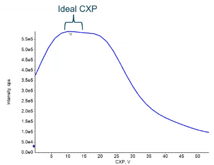 Typically, if you’re choosing a value within the default range 10 to 15, you’re going to be almost at an optimal value right from the start. And in that case, that’s what we see here. So somewhere between that 10 - 15, maybe a value of 12 would be the optimal sort of point to give us the most sensitivity. So what I like to tell folks, when they’re when they’re doing combat optimization, is if you need that little bit of intensity, to get to your limit of quantitation, or limited detection, 60 can help if you’re talking about a few percent. But if you need more than that, going after something like collision energy to declustering potential, or some other way to gain that sensitivity is going to be a little bit more fruitful for you.
Slide: SCIEX OS Software guided MRM optimization #
And all of this, of course, can be done automatically. So in most software’s like SCIEX OS, we have an automatic script, that’s going to go ahead and just go through this process for you. That’s great, especially if you have a lot of compounds. So you don’t have to do it manually, which can be a little bit tedious. The reason I kind of bring this up is even if you are choosing an automatic workflow, which again, great, you just want to be a little bit awary, since we are using something like a syringe pump to actually introduce the compound into our mass spec. Every once in a while I’m guilty of it. I’ll leave a bubble behind in my syringe, and I’ll get a spike in intensity. And that can be a little bit confusing sometimes for software’s. Because they might think, hey, that spike is actually the most intense point really, it’s just an artifact for me not doing a good job in bubbles on my syringe. So if you do choose one of these automated approaches, just go ahead and give it a glance over make sure you’re still paying attention and using some of the rules we talked about to decide if this data is good data.
Step 2: Chromatography #
So we set up our compound optimization, our next topic we need to cover is chromatography.
 So this is really important. So unlike before, we now have our LC in the mix, so we’re no longer just infusing from a syringe. So we’ve got a sample that contains our standard. And we’re gonna go ahead and inject it onto our mass spec. And when we do this, our goal here is to go ahead and choose a column, we need to choose a mobile phase which includes a modifier. And then we need to use that chromatography and when I say use that chromatography, I mean, optimize it. So go ahead and move interferences or separate our interferences from our ions of interest, get our ideal duration, etc.
Slide: Choosing a column #
So how much of a difference does a column make? So in this example, I have Irganox 1135, which I ran on the same instrument with the same mobile phase, same sample, the only thing I changed was the column.
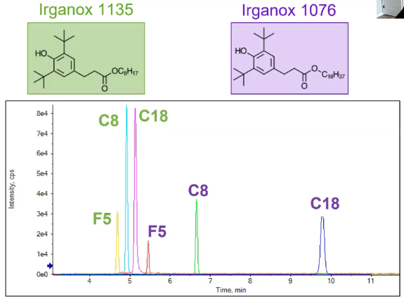 And what we see I’ve got an F5, C8 and a C18. From F5, I had less intensity than my C8 and C18. And with my C8, I had the compound eluding a little bit earlier. And I also didn’t have some of that tailing that was occurring with the C18. So that’s great. Not a huge difference. You could kind of argue between the C8 and C18 to get a similar result. But when we look at a larger compound like Irganox 1076, so the difference here would be that much longer. alkane tail going from a C8 to C18. We see a big difference in retention time. So between that C8 and C18. There’s several minutes I could optimize my chromatography, sure. But I have a really nice peak for my C8. And this might be what you’re after, you might really want that much separation, maybe you have a bunch of polymers you’re looking at, and you really want them spread out. In my scenario, when I was doing this experiment, that’s not what I wanted. So I rolled out the F5, just because of that intensity, but I ended up choosing that C8, because it gave me enough separation between the ions I was interested in. And then I can kind of shorten up the method. When I use my chromatography, like we’ll talk about,
Slide #
well, what are some of the common sort of starting and stationary phases that you can use? So when we talk about stationary phases, if you remember from the first section, we’re talking about selectivity, and selectivity is really going to impact our chromatic resolution.
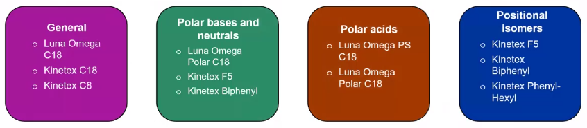 So kind of like what we saw in that earlier slide. Even the difference between a C8 and C18 led to a big difference in my retention time. So which stationary phase you choose is going to depend a little bit based on your goals, but also, it’s going to be heavily impacted by what compounds you’re interested in. So if you’re doing something like positional isomers, something like a by phenol, especially if it has a bunch of greens, can be really useful. Versus if you’re doing something a little bit more polar. And I should have said earlier, I’m really talking about reverse phase chromatography. That’s what I’m going to focus on. So I’m not really talking about HILIC very much. But if you have questions, feel free to ask. So we’re gonna be talking about the reverse phase. So if I have something polar, so my polar compounds earlier, right, something like Luna Omega Polar is a really nice option. This is a C18, but it will retain sort of things like diminish, add or activate some of these really small polar analytes, a little bit better than just a traditional C18. But if you’re just starting out, and you’re totally unsure, starting with sort of just the general C18 approach, it’s a really good starting point, you’re going to get an idea of what’s retaining what’s not retaining, you can even start to experiment with some mobile phases. And then if you need to go ahead and do some optimization on your stationary phase later, or you might say this is just acceptable.
Slide: Column Length #
But beyond the stationary phase, what other variables can affect my chromatography, and one would be column length, right. So as our column gets longer, our pressure typically goes up, which can be totally fine, you’ll definitely want to make sure your system your LC system can handle that. So if you have just a standard HPLC, you want to make sure your pressure isn’t exorbitantly high as 12,000 psi or something like that, where you’re going to damage your instrument. But usually with column length, you’re not too worried about that, but more comes into play with particle size. That being said, if you’d feel that way, a couple of tricks that you can do to sort of reduce your pressure would be to turn up the column oven. So as you increase the temperature in your column up and your pressure should come down. The other option, obviously, would be to go ahead and reduce your flow rate. But what else this column might change. And the big variable would be the elution time. So this might be good or bad, depending on your goals. So if you are really concerned about speed, you want a really quick method, you need separation, but you want your method to be a few minutes long, something like a 50 millimeter column can be a really good choice. That being said, if you want optimal sort of resolution, choosing something a little bit longer, like 150 millimeter column can be a good choice. So if you have a really dirty matrix, having that resolution might be beneficial, because you have a bunch of plant metabolites in the sample that you need to separate from your pesticides or other metabolites.
Slide: Column particle size #
And besides column length, particle size is the other sort of big contributor to our chromatographic resolution. So as your particle size decreases, our pressure is going to increase. So if you want to go with a really, really small particle size, you should expect to have fairly high pressures. So we call that ultra high pressure. So those are things like 10 12,000 psi versus your standard HPLC, which be operating in the 3000 psi range, typically. And what’s the benefit here? So the benefit is, as you make your particle size smaller, typically you make your peak widths, more narrow. So if you think of the same amount of area under your peak, but you’re making it more narrow, it’s coming up and up and up. So you’re increasing your intensity or you’re sort of making a bit taller separating it from its baseline, so you get a little boost in sensitivity. There’s obviously going to be trade offs here. One of which I have felt I’ve come to a future times, but I’ll give you one example of a story. So I went ahead and injected. Well, I got a very nice 1.3 micro meter column from the folks at Phenomenex. They sent it to me. And my goal was to look at some pesticides in this really nasty plant matrix, and have doing this on a 3.5 micrometer column for a while, and everything was going well, but I wanted a little increase in sensitivity. So I went ahead and conditioned my column, and injected my sample onto that column and destroyed that column. Completely destroyed, it was never used again, couldn’t use it. And that happened, because it had this really nasty matrix, right? It was acceptable to use that 3.5. So I had a little bit bigger particle size, but when I got to that really narrow, or tiny particle size, I ended up just clogging it pretty much instantly. So if you’re dealing with sort of these really nasty matrices, whether that be serum or hair, or plants, just make sure that you’re thinking about your sample prep when you’re choosing your column and your column particle size.
Slide: Mobile phase #
So we’ve chosen a column, let’s go ahead and say we chose middle of the road, we got to see your team 100 millimeters with a 2.6 particle size, micro particle size. So just straight middle of the road, the next thing we need to do is go ahead and choose our mobile phase.
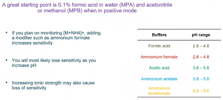 So when we talk about mobile phase, we have our mobile phase A rate that is aqueous, and our mobile phase B for that organic. And usually in LCMS, there’s not a whole lot of playing around we do with our mobile phase in the sense of it’s A is pretty much always water, B is usually methanol, or acetonitrile. most labs would prefer methanol because it’s it’s quite a bit cheaper than acetonitrile. But sometimes acetonitrile gives you a little bit better resolution, where there is a little bit more flexibility would be in your buffers, or modifiers. So here, we have some examples of some common modifiers. In positive mode, I’d say formic acid is almost the most common modifier, and we’re heading modifiers to accomplish a few things.
One, is we want that pH control, right. And we want that pH to be stable, we don’t want to have shifts in pH that are going to cause resolution differences or illusion time differences. So we want that stability, and
Two, is we want that pH to be different than the pKa of the compounds we’re interested in right, as the pH and pKa. get very close. If that pKa is the same, right, we’re not really not going to be ionizing efficiently. So as we move that away, we ionize a little bit better. So typically, we will go into the two to three pH range for most compounds, and positive mode seems to work pretty well. One thing you’ll also notice here is all of these buffers are volatile. So we don’t want to use salts, things that maybe were acceptable with LCUV, like a phosphate buffer. Because we needed to qualify as we’re doing a different experiment, we need to have things enter the mass spec ionize where set up different and we’re looking at different things, we’re not doing UV analysis anymore. So something like a phosphate buffer would be just inappropriate. And if you’re unsure, almost always go ahead and just try a generic starting mobile phase first. So something like water with some formic acid, usually 0.1% is a really good starting value. And you can add it to your organic as well. So something like a 0.1 in your methanol, if you are interested in things like ammonia adducts. So for example, on this slide I showed earlier with that, you know, huge ammonia adduct peak, and is something like ammonium formate is going to help promote that adduct for me. So if you are looking at ammonium adduct, adding ammonium formate is going to be your best bet. And you’re gonna want to make sure that you’re doing this regularly, right? These things are volatile. So as we let them sit, our mobile phase, essentially it gets called Old. But we’re just losing our our modifiers and buffers. So if you notice, for example, the sensitivity of certain ions decreasing over time, and you look up on your LC stack, and you see that you’ve been using the same mobile phase for a month now, it’s probably a good time to make a new batch.
Slide: Gradient #
So we’ve chosen our mobile phase, we’re just going to go generic again. Now it’s time to sort of use that chromatography and get the method to meet our standards and the things we need to accomplish.
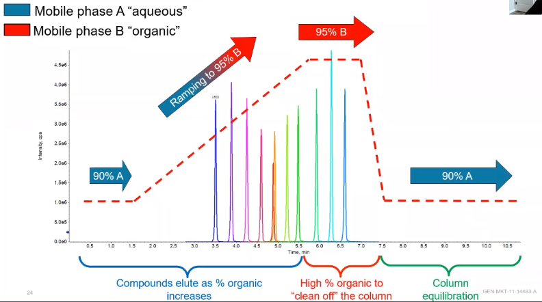 So we talked about this a little bit last time, so I won’t go too far into it. But we essentially have these four stages of chromatogram. We have a aqueous stage where we’re letting our more polar things elute, we have this ramp stage. And then we have our non negotiable final two stages, which be a stage where we clean off the column, or we hold at a very high organic. So typically, this is 95% or above our mobile phase B. And we want to hold there long enough to get ideally three column volumes worth of mobile phase through our column to really clean that out. And finally, our equilibration phase, which is also non negotiable, we need to get our starting conditions back at the exact same place they were when we did our first injection, so we don’t have shifts in our attention time. And here, we would just go ahead and hold for the same three column volumes. But how do we use this chromatography, because certainly, it’s not always going to look like a ramp up from 95%, sometimes we may be are holding for a little bit to let some separation between some isomers occur. Sometimes we might run super fast, or just have an isocratic method.
Slide #
So what are we doing when we do that, and essentially, with reverse phase chromatography, as we increase the percent B, things are going to lead faster.
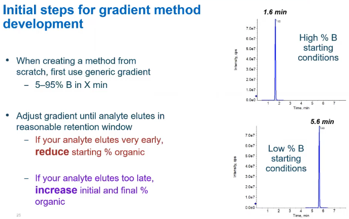 So if we increase that ramping, or we increase that starting condition, so here I have the same compound, the only differences, I have a high starting condition, for my percent B versus a low starting condition on the bottom. And you’ll notice the retention time is very different. So about four minutes different. So this could be great if I’m looking for a really fast method for this specific compound. But if I have things are maybe super polar, and I started at a very high organic, it just won’t be retained by my column at all. And it will just kind of fly through the system, and it won’t have a nice peak. So there’s going to be a little bit of a balance. And that’s like that with everything with method development, right? We’re talking about building a customized method for your analysts. So it’s going to be very custom.
Slide: sMRM methods #
[32:08] And finally, once we’ve kind of identified that, yes, this is, this is my chromatography, I’m happy with, I want to go ahead and move on to my final stage, the next thing I would encourage you to do is go ahead and schedule that method. So scheduling means that you’re essentially telling the software in your instrument, a time to look for that analyte. So you’re saying at two minutes is one analyte, in this case, four minutes at around four minutes is where I expect this analyte to show up.
And it does great, why am I doing this, the reason I’m doing this is, because if I don’t schedule my method, and I have a ton of different analytes, it’s going to be looking for everything all the time. And if it’s looking for everything all the time, it can’t do as good of a job. Similar to me, if I’m multitasking, I can’t do as good a job. Whereas if I’m focused on one thing and a specific time, usually can do a little bit better. So you’ll see that in your data quality. So if you only have one or two main analytes, maybe a handful of analytes, it’s less important. But if you’re getting into the range of 20,30, 40, or you know, a few 100 analytes, that’s for scheduling really becomes not only important, it’s pretty much mandatory. And the differences in the data quality can be seen here. So we have the pink, which was unscheduled, and the blue, which was scheduled. And what you’ll notice about the pink is that it’s essentially a triangle. So each one of those dots represents a data point where the instrument actually collected data. So we’ve got this triangle sort of shapes. And that triangle becomes really difficult to integrate, because it’s going to change a lot depending on where that apex is. So it’s going to change depending on where the instrument was what it was looking for, at that time, compared to our peak in the blue, where we have this nice sort of Gaussian peak with plenty of points across it. So if there’s a little bit difference in where those points are, it’s not really going to change the area underneath my peak as much as it would if I was just integrating the triangle. So typically, we’re going to aim for somewhere between 10 and 15 points across our peak, that’s a really good range to be in. And 12 would kind of be that sweet spot. Goldstar. Yeah.
Slide #
And it’s really easy to do, once you’ve determined your chromatography is what you want. We’ve already done all the compound optimization, you just run a standard, go ahead, copy retention times and paste them right back into your analytical method. And you’re ready to go. You have your scheduled MRM method so easy is that you get a lot of benefits in terms of data quality.
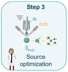
Step 3: Source Optimization #
So are we happy with our chromatography we’re happy with our comment up? Last, we have to optimize for our source conditions.
Slide: On-column source parameter optimization #
So the way I’m going to show you how to optimize for source conditions might be a little bit different than what you’re used to. This is my preferred method is called on Column source parameter optimization.
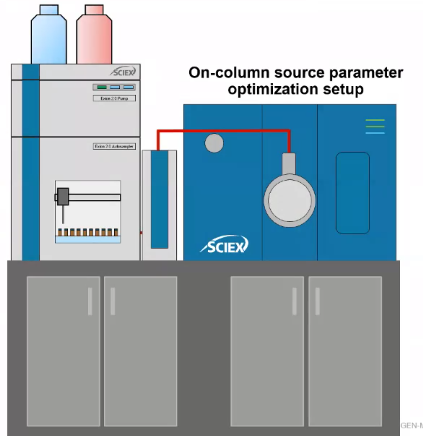 The real difference here is that I’m not infusing anything. So in the past, maybe you used a column split T’s. But essentially what you’re doing is using a syringe pump to infuse your compound of interest. And then also, using your LC, to sort of introduce your mobile phase. Here, what we’re doing is we’re taking a sample with our standard with all the compounds we’re interested in. Since we know our chromatography, and we’d have them optimized, we’re just going to inject it. And we’re going to try basically a ton of different source conditions, and we’ll get the optimal one.
Slide: Optimize five parameter of ion source #
And the reason I like doing this is because when we look at the parameters that we’re optimizing, it’s going to be really dependent on flow rate and mobile phase composition.
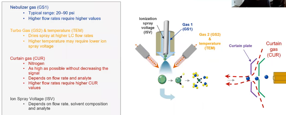 So we talked a lot about our source conditions last time in the sense of what they are. But just to kind of briefly reintroduce them, we’re going to be optimizing for these five parameters, primarily our
 GS1, which is what’s going to help us create that nice spray, that’s going to let us ionize our compound, we have our GS2 and our temperature, these kind of work in tandem. So we want to promote evaporation. So we’re going to use a little bit of gas to help the evaporation in addition to our temperature, obviously, to help that. And then we’re also going to do our curtain gas (CUR), that’s what’s keeping our instrument clean. So that’s that gas coming out from behind our curtain plate. That helps keep all those neutrals and other things that we don’t want in our mass back out. And then our iron spray voltage (ISV). So this is the actual voltage we’re applying to promote that ionization. And since these kind of depend on our flow rates, they depend on our mobile phase composition to a point, I like to do an on column. And one example that I have is I was working with a lab that was doing some cannabis analysis. And they did their source optimization, everything looked good. They’re doing it by just refusing their standard. And they had their LC set to 50-50 in terms of 50%, water, 50% ethanol. And then when they went to actually run the method, what they noticed is they weren’t seeing any peaks in the beginning of the chromatogram. And they’re having a really hard time figuring it out. So fill out there and that what was happening was essentially, kind of easy to see. Because if you looked at the source, they were essentially just washing their curtain plate, they had set the temperature so low, because they’re using more organic when they did their optimization, that when they did their starting conditions, which was 100% water, all the water was just rinsing off the curtain plate, going into their source exhaust and causing them a bunch of issues. So just my little example of why I choose to do it this way. And I think it’s easier to
Slide #
so we’re gonna go ahead and tell our instrument what we want it to run, in a sense, we tell it the chromatography method that we’ve already developed, we tell it the compounds it’s going to look for with their optimized parameters.
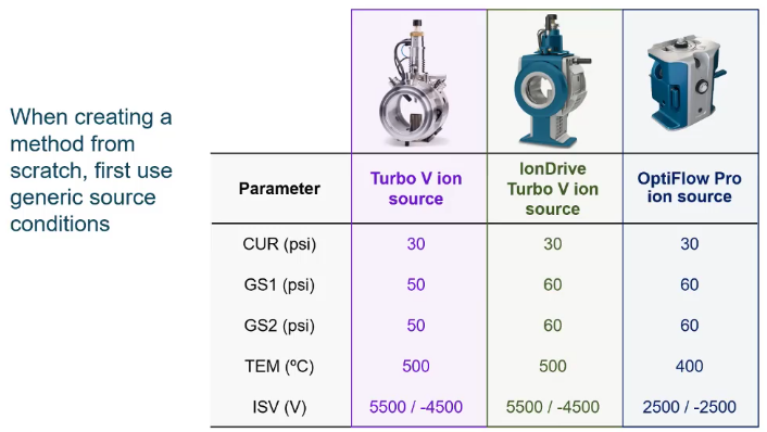
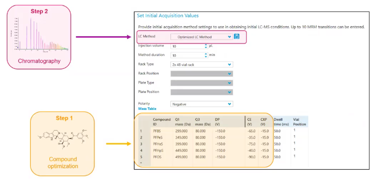 And then we’re just going to choose some generic source conditions. So these will vary a little bit depending on the source that you have. But here’s just some of my sort of generic starting conditions. And really, it doesn’t make a difference. As long as you can see the compounds you’re interested in, we’re going to optimize for these.
 So if you can see the compound you’re good to go. Don’t worry about it too much.
Slide #
So when we do optimize for these conditions, what are we doing, we’re going to go ahead and inject that sample, and we’re gonna inject it a lot. So I like to set this up overnight. And we’re basically going to put it through the paces and run all the conditions we want.
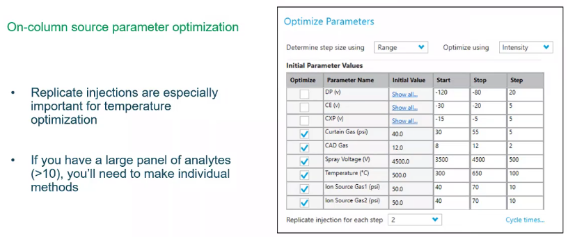 So for curtain gas, for example, the minimum curtain gas I would run on a method would be about 30 psi. But I’m going to go ahead and inject my standard at 30 psi, I’m going to inject it again at 35 injected, again, pre injected again at 45. And then plot the data. So when I plot the data, I should see maybe an increase maybe 45, that gives me the most intensity, versus 35, etc. And when you do that for all my variables, so inside, so so there’s a nice little script that will do this for you. You can do the same thing and analyst as well. But if you have a lot of analytes, sometimes I’ll just make the methods and just change the variables myself. It kind of depends a little bit on your personal preference.
Slide #
So here’s an example of what that looks like. So I have Avermectin here. And I have different iron spray voltages.
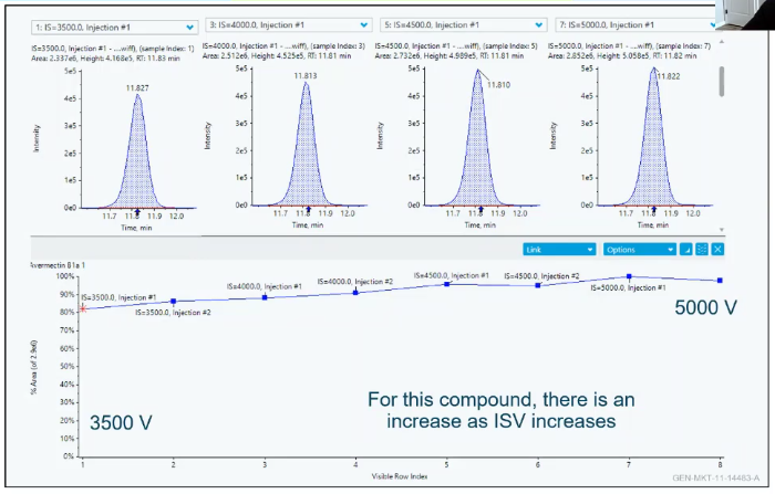 So I’m starting at 35 down here, and I’m moving up to 5000. And what we see is sort of this increase in area as we increase that voltage. So what you’re probably thinking is that might be true for Avermectin but what if that’s not true for something else in your panel, if you’re looking for more than one thing, and that happens, that happens a lot. And what you end up having to do is make compromises. so Avermectin I like to show because it’s very temperature sensitive. So it looks a really really low source temperature compared to something a different pesticides like pyrethrins, which like a really warm or hot source temperature. So I’ve kind of got to choose a middle ground. And since I struggle with my sensitivity on my Avermectin, I choose to use a lower source temperature. And those are kind of some of the hard choices that you’re going to have to make when you make your own method. But you can plot all of them, get an idea, choose your best values, and then you’re good to go.
Slide #
So method development, whether you’re adding a compound, or you’re building a method from scratch, it should be pretty straightforward, you follow any steps, but you can see there’s a lot of flexibility in all of those steps, there’s going to be a lot of choices that you need to make, that are going to be specific to your goals. So just like always encourage you to think about your goals first. So if your goal is to have the fastest highest throughput method, you’re gonna make some different choices than if your goal is to have the most resolution. So if you are in a government lab, where you maybe want to separate isomers, for some research purpose, you might want to choose a really long method. And that’s fine. Versus if you are in a lab, and you’re running customer samples, and you need to turn around and make a profit. Running a shorter method is going to be more important to you. So just ask yourself, what your goals are, and why you’re or what you’re trying to accomplish with your method.
Slide #
But regardless, go ahead, plan ahead, that development takes time. And since we live in a world where there’s a bit of regulation, which we all know, once we validate a method, it becomes very hard to change. So make sure that you’re happy with your method from the beginning. And taking notes is also my my next biggest push. So if you have those five fragments, for example, all recorded in the future, when you go to do your chromatography or inject your first Matrix sample, and you notice there’s a huge interference, you haven’t wasted any time, you can just go back to your notebook or your other method and pull a new transition. So take the notes, and take your time during these method development stages.
Slide #
And if you are interested in sort of the step by step approach, if you want to know how to optimize a compound, where to click when you click, SCIEX Now Learning Hub is a great tool. We also have some courses open now on our sites. So you can come out that’s actually what I did a long time ago, when I first started doing some QToF analysis, flew out to the safe sight and did their training. And I really enjoyed it. So check out the Online Learning Hub if you’re looking for those more sort of step by step instructions. And with that, if there are any questions, I’d be happy to answer them.
Q&A #
Q#1
Thank you, Karl, for sharing that great information. And now we will move on to the question and answer session of the presentation. We have some questions about source optimization, Karl, and you were discussing optimizing the source. What’s an approach if you have five or six unique analytes, Or more analyzed with different chemical properties? And how do you go about source optimization when looking at different classes in one methodology?
Yeah, it’s a great question. So when I do source optimization, regardless, if I’m looking at two analytes, or if I’m looking at 150 analytes, I really take the same approach. And I really liked that on column approach, because I can add everything to the MRM method, I know when these things are eluding. So as long as I choose sort of generic source parameters, where I can see all of those compounds, I’m going to go ahead and step through each one of those sorts of different variables, GS1, GS2, temperature, etc. Until it to find an optimal value. But if your question is more, how do we make those tough choices? You know, sacrificing one’s intensity for another? I think the real answer is you have to look at the limits that you’re trying to hit. So what is that lower limit that you want to hit or need to hit if it’s regulated? And make sure that you’re achieving those in those difficult compounds first.
Q#2
Excellent, insane light a compound optimization when you’re doing infusion? Should you be running mobile phase at the same time, or should you be working purely from infusion standards?
Really good question. And that actually has come up quite a bit with customers in the past. So what I typically like to do is when I prepare that standard for infusion, I’ll actually use my mobile phase to make that dilution. So I’ll take my neat standard and I’ll dilute it into my mobile phase. So you can do have 50-50 of each if you want, or you could just do your organic if it has some formic acid. But you’re absolutely right, you want some of that modifier in there to prove out that ionization, like we talked about.
Q#3
Excellent. The next question is around, what do you perform the source optimization at towards the end? You talked about kind of reoptimizing at the end of why do you do it in that specific order?
Yeah. And the reason being is that, that’s kind of where it falls, right? Because for my compound optimization, I don’t really need any information about source conditions. There’s no chromatography. So I can do that first. So that’s why we choose to do that first. And we’ll need that those compound parameters in order to do our chromatography, right. So we’ll need to choose our compounds, optimized for them, etc. And for source optimization, if you’re doing the on column approach, you’ll need both the chromatography and those compound parameters. So it’s kind of just where it falls in the process of things.
Q#4
Excellent. Also, you’ve discussed matrix interference and suppression, how do you go about determining if you’re experiencing suppression? And if so when do you get indications that you should adjust your chromatography to account for that?
Good question. Great question. And some of the clues. So there are a few different clues that you’re experienced depression, and suppression can happen in a few different ways. Right. So one way I’ve experienced it quite a bit is actually in the source. So I have source depression. And one of the big clues that I’m having an issue with source depression is if I run a calibration curve, and I have my internal standard in there, and as my concentration and my calibration curve increases, I’ll start to see this decrease in my internal standard over time. And that’s because there’s only so much that can be ionized at the same time, right and my source. So essentially, my internal standard and my compound of interest, or my analyte, that I’m actually measuring, are competing for that ionization. So I get some source suppression. That source suppression can happen with internal standard, of course, but it could also happen with anything in the matrix as well. So if you’re seeing something like that, one option is dilution. Dilution can really help with suppression and matrix interferences.
Q#5
Excellent. We have some questions around column choice as well. And the first is around does column choice and column chromatography, change and impact intensity?
Yeah, yep. So kinda like what it showed in the example with Irganox, 1076, and 1135. You saw that difference in intensity between the F5 and the C8 and C18. So it was just not doing as good of a job selecting for that compound. So you will see differences in intensity, for sure. And then when we get into things like a particle size, and even column length, that’s where you can also see changes in intensity. So it might be the same stationary phase might be just to C18 like the other C18, but if it has a smaller particle size, you’ll likely see a more sort of narrow, intense peak than larger particle size.
Q#6
Excellent. As we know, there is a tolerance for retention time, do you have any rule of thumb of how you might select or set your retention time tolerances for a method?
Absolutely, I usually default to the sort of old adage of plus or minus point one seconds, or point one minutes, so I’m sorry. So about six seconds, that’s usually my acceptable sort of wiggle room in terms of my my peak actually shifting. But what I might do if I’m setting up a scheduled method is sort of broaden or make that window a little bit bigger than that, in case something does happen. So you know, maybe this one sample prep method was a little wonky, or something happened, something occurred got really hot in my lab, and my mobile phase warmed up a ton and my retention time started to shift. For my window that I’m looking at, I’ll usually allow it to be about 20 seconds.
Q#7
Excellent. The next question is around data points and data quality, how many data points do you generally require or suggest to ensure reproducibility and high data quality?
Yeah, so 10 to 15 is sort of that good range for points across the peak. And then 12 would be the ideal area or the ideal range to be in mid value. And the way we’re kind of determining that or the way to determine that would be to go ahead, look how wide your peak is. So I’ll do easy math, because It makes it easier for me. If your peak was 10 seconds across, we want to have our cycle time to be roughly a second. So if our cycle time was a second, we will get 10 points across our peak. So the amount of analysts you have is kind of going to dictate, because I did see that question about 12 volume, or dwell time is going to dictate that dwell time. So they kind of is an interchangeable play. But usually you want to adjust your cycle time accordingly to get enough points across to be.
Q#8
excellent. The next question is also in regards to dwell time. And how big of an impact does dwell time have on analytical sensitivity and intensity of a given peak?
Yeah, it can have a big impact. So I didn’t mention it. But typically, we want to make sure our dwell time, in a perfect world, somewhere around 50 milliseconds would be great. Obviously, that’s not achievable for everything. But we really don’t want to dip too much below sort of 10 milliseconds, because when we do, we’ll start to see sort of variability in our peak intensity, and also just a little bit less intensity. So if you think about it from just like a very high level, right, we’re giving the instrument more time to do something. And as we give him more time to do something, it does a better job. So if we can get into that 50 millisecond range, we’re in a really nice spot in terms of our data quality.
Q#9
Excellent. We have another one in regards to chromatography optimization, and, uh, you know, wide panel or large panel. So if you have a sample that contains analytes, with a wide range of pKas, maybe anywhere from three to nine in the specimen, how do you determine what’s the right pH to provide optimum chromatography? Or what’s the strategy for that?
Good question. And that’s a tough position to be in for sure. It’s going to depend a little bit, I’d say what ionization mode you’re using. So it kind of comes this area of what fits best for most. And you can do other things. So for when I do polymer analysis, for example, I will add formic acid, and I’ll also add ammonium for me, because I have two goals. One, I want to promote ionization, but two, I’m almost always looking at that ammonium adduct. So I want to make sure there’s a nice healthy supply of ammonium in my sample to kind of promote that adduct for me. So that might be an option, that you can go ahead and try adding two modifiers. If that’s kind of your goal, but in general, I would say go ahead, try something like formic acid, which is going to work for the majority of things and kind of assess where you’re at. If there are a few compound classes that are giving you trouble. That’s where you might kind of get into that range where you can say, hey, maybe I’m going to try something different.
Q#10
Excellent. We have a couple of questions about mobile phases. The first is, is methanol preferable? How do you choose between methanol and acetonitrile?
Yeah. The the correct answer would be to try both and see what happens. But if that’s not an option, there are some advantages of methanol over acetonitrile, methanol one would be less expensive. So if you’re talking about a cost per sample basis, maybe that’s where you make your choice. And then typically, acetonitrile is a little bit stronger. So if you’re dealing with sort of this more nasty, difficult complex matrices, acetonitrile will do a better job cleaning off your column and also give you a little bit more resolution.
I would again like to thank you, Karl, for the informative presentation. And thank you for joining us today. We hope you found the presentation informative, and we look forward to seeing you at the next LCMS 101 session.